Evaluating Retrieval Without Ground Truth

A graph-theoretic approach to building reliable LLM judges for retrieval and ranking

Recently, we have been spending a significant amount of time optimizing semantic retrieval pipelines across retrieval-augmented generation (RAG), threat detection, code search, legal search and recommendation systems. We keep hitting the same wall: a lack of ground-truth labels.

In threat detection, raw data can be highly sensitive and often cannot leave the customer’s environment, making external labeling a non-starter. In healthcare and legal, labeling needs domain experts, and privacy rules narrow the pool of experts you are allowed to use. Even in less regulated domains, from what we have seen, building a sufficiently large labeled dataset can take weeks of expert time per evaluation cycle, during which the labels can go stale as the product evolves.

The retrieval layer dictates what the downstream model sees, so getting it right is important. In the ML community we already have metrics for measuring this: Normalized Discounted Cumulative Gain (NDCG), Mean Reciprocal Rank (MRR) and Recall@K. Each of these metrics needs a pre-existing ground-truth set of query-document relevance judgments. In domains such as the ones discussed above, these ground-truth judgments can be prohibitively expensive to obtain.

We try to answer this question here: how do you evaluate a retrieval system when you don’t have ground-truth labels?

Similar Is Not Always Relevant

An obvious first move here is to skip labels altogether and use a modern embedding model on the query and the retrieved documents, and take their cosine similarity as the relevance score. But it doesn’t hold up. The problem is that what “similar” means to the embedding model is rarely what it needs to mean for your task.

Consider a threat detection example: Two emails might share 90% of their tokens (corporate boilerplate, signature blocks, legal disclaimers), yet one is benign while the other harbors a novel credential-harvesting payload. A retriever scoring purely on textual overlap will likely treat them as near-duplicates. The same problem appears in code search: two functions can be lexically near-identical but can execute entirely different logic, while two implementations of the same algorithm in different languages share almost zero tokens.

The issue is structural. Embedding models are trained to approximate generic semantic similarity from large, mixed corpora. They are typically unaware that in your specific domain, “relevant” means “same attack pattern,” “same algorithmic behavior,” or “same legal doctrine.” Their notion of similarity is frozen at training time, while your notion of relevance is specific to your task.

What we need is a qualitative judgment: Given this query, is Document A more relevant than Document B for the underlying task? That kind of judgment requires deep contextual understanding and the ability to apply a task-specific definition of relevance. This is where frontier LLMs have demonstrated a real edge: Thomas et al. (SIGIR 2024) showed LLMs can accurately predict searcher preferences, suggesting the same capacity generalizes to domain-specific relevance calls.

By using an LLM as a judge, you can pass it the query, the candidate documents and a rubric—a plain-English specification of what “relevant” means for the task.

For example, a rubric for a threat-detection retriever might say: “A document is relevant to the query if it describes the same underlying attack pattern (e.g., credential harvesting, lateral movement), regardless of surface-level features like sender domain, boilerplate text, or formatting.”

Importantly, this approach sidesteps much of the labeling bottleneck. There is no pre-built, ground-truth dataset to acquire. The rubric is your spec; the judge is your labeler.

The LLM Judge Just Needs to Be Reliable

A common pushback to this approach is: “How can we trust an LLM as a judge for relevancy? Our problems are sophisticated and domain-specific. An LLM won’t understand the nuances.”

Indeed, Soboroff (2025) argues that using LLMs to generate relevance labels caps your evaluation at the judge model’s own ceiling. They treat it as a categorical mistake to substitute LLM judgments for human ones.

This is an important concern when LLM labels are taken as absolute truth, used to certify a system’s final quality or to compare against published benchmarks. Our use case is narrower. We believe that the judge does not need to be flawless. It needs to be a reliable enough yardstick to spot where the retriever fails, iterate and watch the metrics improve. On that bar, recent evidence is encouraging. The SIGIR LLMJudge benchmark (Rahmani et al., 2025) evaluated 42 LLM-generated label sets from eight teams against TREC 2023 Deep Learning judgments, and found that LLM judges preserve system rankings (high Kendall’s tau against human-derived rankings) even when their per-label agreement (Cohen’s kappa) is weaker. We believe that is exactly the property an iteration loop needs: you may not get the exact relevance score right, but you can still tell which retriever is better.

In our view, an LLM is better suited than an embedding model for four specific reasons.

• Full cross-attention over query, document and rubric. Embedding models are bi-encoders: query and document are encoded independently into fixed vectors with no awareness of each other, and relevance is approximated by a dot product. Cross-encoders attend jointly over the pair, which is why they work as re-rankers, but they’re trained on a fixed notion of relevance and can’t be steered toward a domain-specific rubric at inference time. An LLM judge processes all three inputs in a single context window, attending across query, document and rubric simultaneously. This is why the rubric isn’t just metadata: it actively shapes the comparison in a way an embedding model’s frozen notion of similarity cannot.

• Inference-time reasoning. An LLM can reason through hard comparisons and spend more compute on them, while an embedding model compresses each input into a fixed-length vector in one forward pass, regardless of difficulty.

• Scale. Frontier LLMs have substantially more parameters than the embedding models they’re judging, which means more world knowledge and linguistic competence available to the judge than is accessible to the retriever.

• Post-training on judgment tasks. Frontier models are post-trained, often with reinforcement learning from human feedback (RLHF), on tasks that explicitly involve comparison and preference. Embedding models are typically trained with contrastive objectives on more domain-targeted distributions (e.g., MS MARCO, BEIR).

None of these reasons make the LLM flawless on a given comparison. Across enough comparisons, though, we believe it’s a reliable baseline for surfacing systematic errors in the retriever.

LLMs Score Poorly But Compare Well

The intuitive first step is to use an LLM judge as a direct scorer: ask the model to rate relevance on a 1–10 scale for each document, then compute NDCG against those scores. This approach doesn’t work well for two reasons:

• Poor Calibration: LLMs are not well-calibrated on absolute scales. The same document might get a 7 on Monday and a 9 on Tuesday. Feng et al. (2025) found that even frontier LLM judges fail to maintain consistent preferences in roughly 25% of challenging cases.

• The Lost-in-the-Middle Problem: A natural fix for calibration is to score all candidates in a single call, forcing the model to rank them against each other. But long lists run into the “lost-in-the-middle” problem: models attend to the start and end of the list and degrade in the middle (Liu et al., 2023). While simple needle-in-haystack tasks show improvement, NVIDIA’s RULER benchmark (2024) confirms that tasks requiring comparison across items in long contexts still degrade in the middle.

What LLMs do well is pairwise comparison: Is A more relevant to Query Q than B? Pairwise judgments work because the context is small and the task is well-posed. Qin et al. (NAACL 2024) confirmed this empirically: Pairwise Ranking Prompting with a 20B open-source model outperformed GPT-4, which has an estimated 50× more parameters, by over 5% at NDCG@1 on TREC-DL2020. But this introduces a new engineering problem: how do you turn a stream of pairwise comparisons into a global ranking?

LLM Judges Aren’t Transitive

Turning pairwise comparisons into a global ranking depends on one assumption: transitivity. If LLM judgments were perfectly transitive (i.e., if A > B and B > C implies A > C), global ranking would be trivial. In practice, they are not.

Xu et al. (2025) studied this exact phenomenon in the AlpacaEval framework, where LLMs judge which of two model responses better follows an instruction. With GPT-4-Turbo as the judge, they found non-transitivity rates of 4–8% across model triplets. With a weaker judge like GPT-3.5-Turbo, the rate jumped to 21–23%.

The non-transitivity rate is highest when the things being compared are close in quality, which is precisely the regime a retrieval evaluator cares about: the top of the ranking, where small differences in relevance determine which document is retrieved.

Because of these cycles, you can’t just throw quicksort at the problem. Feed a standard sorting algorithm a loop, and the final ranking you get is largely a function of which comparisons happened to execute first.

A Graph-Theoretic Solution

We believe a solution to turning non-transitive pairwise judgments into a reliable global ranking is to treat the comparison results as a directed graph, an approach formalized in Contextual AI’s BlitzRank (2026).

1. Build the graph. Rather than ranking all N documents at once (lost-in-the-middle) or comparing them pairwise (quadratically expensive), do it in batches. Treat each document as a node. Show the LLM k candidates at once (say, k = 5) and ask it to rank them. That single call reveals k(k−1)/2 pairwise edges, or ten relationships for the price of one when k = 5.

2. Transitive closure. If the graph contains A → B and B → C, infer A → C for free. No additional LLM calls needed.

3. Handle the cycles. A non-transitive cluster (A → B → C → A) becomes a strongly connected component (SCC). Instead of breaking the cycle arbitrarily, collapse those items into an equivalence class: a “tier” the system treats as tied.

4. Schedule the next batch. A single k-wise call only ranks k documents, so you keep running batches until every document’s tier is pinned down. The trick is choosing which k to query next: pick documents whose position is still ambiguous, meaning ones inside a non-trivial SCC or not yet compared against enough others to anchor their rank. Every batch either resolves a cycle or settles an unfinalized node. All edges land in the same graph; there is no separate merge step.

If you contract each SCC into a single node, what remains is a directed acyclic graph (DAG), which admits a topological order. Your output is a sequence of relevance tiers.

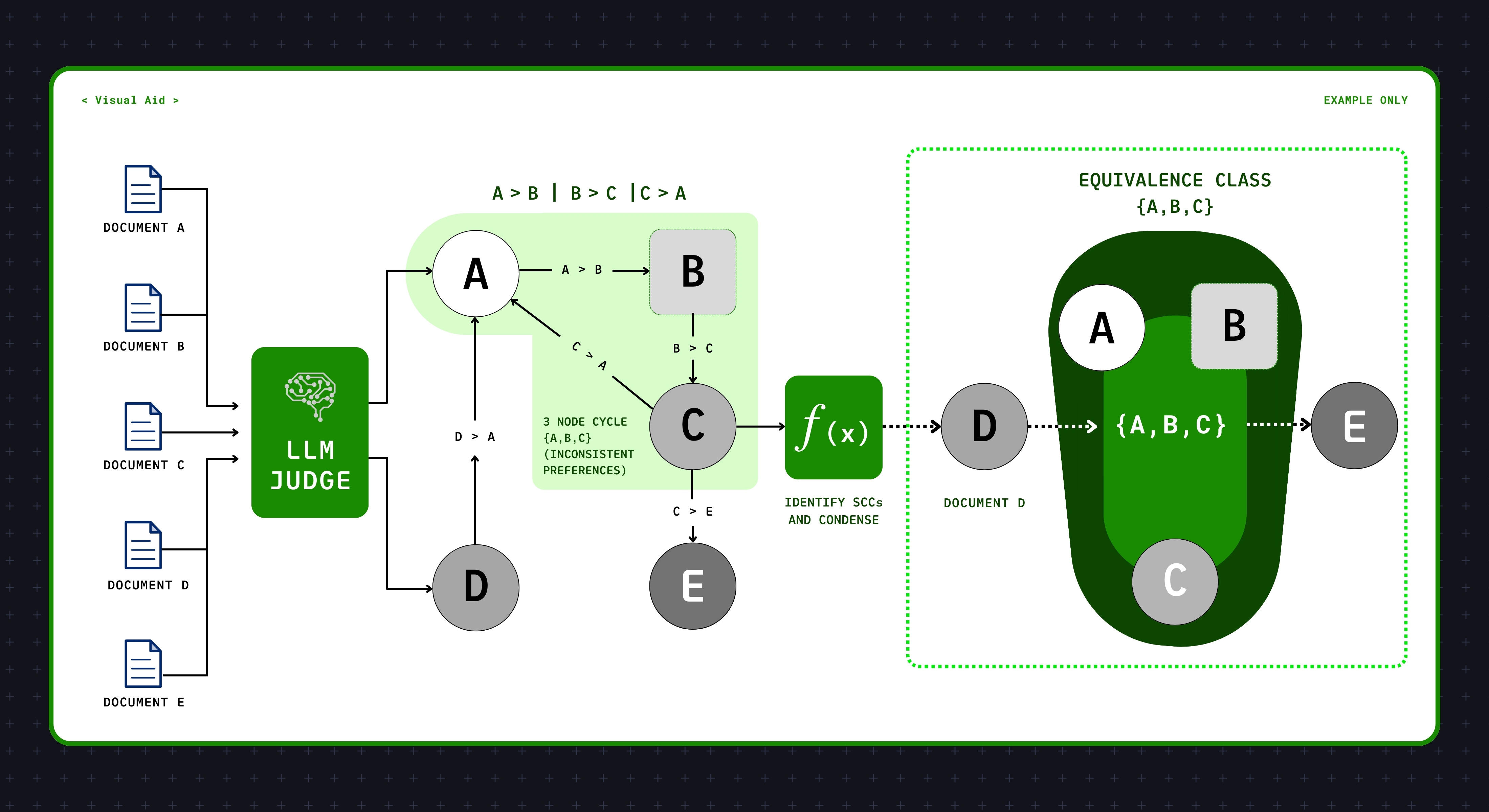
BlitzRank applied this approach across 14 benchmarks and 5 models, achieving strong results across the benchmarks tested: matching or exceeding accuracy while requiring 25–40% fewer tokens than comparable approaches, and ~7× fewer than pairwise reranking at near-identical quality.

Other tournament-style approaches exist. Xu et al. (2025), referenced earlier, propose round-robin tournaments combined with Bradley-Terry preference models to handle non-transitivity from a different angle. The core mechanics (k-wise queries, transitive closure, SCCs as tiers) generalize across all of them.

From Graph To Retrieval Metrics

Recall the original problem: we want to evaluate a retrieval pipeline but have no high-quality ground-truth data to evaluate against. We believe the tiers solve this. For each query, the graph yields a relevance-tiered ranking of your candidate pool that stands in for the human labels you never had.

From there, the evaluation runs as normal. Compute NDCG@K, MRR, recall@K against the LLM-derived tiers. We get a metric we can iterate on, the same way we would against human-annotated labels. NDCG@K is a particularly natural fit, since ties are first-class outputs of the SCC contraction step.

Notes From Practice

The rubric is doing more work than it looks like. It is the working definition of relevance for this evaluation. If the judge keeps disagreeing with your intuition on specific cases, the rubric is usually where to look first, before you start tinkering with the judge.

For higher fidelity, use a small ensemble. Run the same comparison through 2–3 frontier models from different providers and take a majority vote. Single models have systematic biases: one might overweight a particular surface feature, another might be overly literal. An ensemble mitigates this.

Ensembles do not escape Condorcet. Majority votes can themselves produce cycles, a well-known phenomenon called Condorcet’s paradox. This is precisely why the graph aggregation step matters even when you are pooling across models. The pooling does not give you transitivity. The graph does.

This is an offline evaluation methodology. The whole pipeline is slow and token-heavy: an LLM call per k-wise batch, multiplied across enough batches to resolve the graph, multiplied again if you ensemble across judges. This is unlikely to scale at inference time. We think it is well suited to the evaluation harness, where you can run it periodically against a candidate pool, measure retriever performance and get the ground-truth-like labels you would not otherwise have.

Closing The Loop

Procuring ground-truth labels in sensitive or expert-driven domains is hard, expensive and often impossible. With an LLM judge and a graph aggregation step you can generate your own labels against your own rubric. The retrieval system you ship next week can be one you have actually measured.

---

Further Reading

• LLM-as-a-judge and evaluation

  • Thomas, P., Spielman, S., Craswell, N., & Mitra, B. (2024). Large Language Models can Accurately Predict Searcher Preferences. arXiv:2309.10621

  • Soboroff, I. (2025). Don’t Use LLMs to Make Relevance Judgments. PMC11984504

  • Rahmani, H. A., et al. (2025). Judging the Judges: A Collection of LLM-Generated Relevance Judgements. arXiv:2502.13908

  • Feng et al. (2025). Are We on the Right Way to Assessing LLM-as-a-Judge? arXiv:2512.16041

• Long-context and ranking limits

  • Liu et al. (2023). Lost in the Middle: How Language Models Use Long Contexts. arXiv:2307.03172

  • Hsieh et al. (2024). RULER: What’s the Real Context Size of Your Long-Context Language Models? arXiv:2404.06654

  • Qin et al. (2024). Large Language Models are Effective Text Rankers with Pairwise Ranking Prompting. arXiv:2306.17563

• Tournaments, non-transitivity and aggregation

  • Xu et al. (2025). Investigating Non-Transitivity in LLM-as-a-Judge. arXiv:2502.14074

  • AlpacaEval. GitHub

  • Agrawal, Nguyen & Kiela (2026). BlitzRank: Principled Zero-shot Ranking Agents with Tournament Graphs. arXiv:2602.05448

  • Pipitone et al. (2025). zELO: ELO-inspired Training Method for Rerankers and Embedding Models. arXiv:2509.12541

  • Condorcet’s paradox. Wikipedia

---

William Barber is a Search Relevance Engineer helping turbopuffer’s customers evaluate and apply state-of-the-art models and approaches to improving relevance in their search pipelines. He was formerly a technical lead for search and recommendations at Guidepoint.

Kshitij Jain is an AI Tech Lead in the Georgian AI Lab, where he helps portfolio companies to implement scalable AI solutions and refine their technical roadmaps. Prior to joining Georgian, he spent five years at Google working on Search Ads CTR prediction models, where he led the team’s resource-efficient ML efforts. You can read more of Kshitij’s writing at his personal substack.

We are grateful to Paul Inder and Kartik Gupta for thoughtful feedback on this essay.

This blog is provided for informational purposes only and should not be relied upon as legal, business, investment, or tax advice. Nothing in this blog constitutes investment advice, nor is it intended for use by any investors or prospective investors in any Georgian funds. This blog may include links to external websites or information obtained from third-party sources. Georgian has not independently verified and makes no representations regarding the accuracy or completeness of such information, whether current or ongoing.If this content includes third-party advertisements, Georgian has not reviewed such materials and does not endorse any advertising content or the companies referenced.

This blog may contain reference to Georgian investments or portfolio companies. Any such reference is for illustrative purposes only and may not be representative of all investments made by funds managed by Georgian. Contact Georgian for more information.